Marcelo Jo

Hi there,

After almost two years of personal hard work, I’m back to share a little about linear regression and gradient descent.

What is linear regression?

From wikipedia

In statistics, linear regression is a linear approach for modeling the relationship between a scalar dependent variable y and one or more explanatory variables (or independent variables) denoted X.

[…]linear regression can be used to fit a predictive model to an observed data set of y and X values. After developing such a model, if an additional value of X is then given without its accompanying value of y, the fitted model can be used to make a prediction of the value of y.

Simple linear regression is when y is a function of a single variable x and multiple linear regression is when y is a function of multiples variables, like x1, x2, x3, etc. In this post we’ll cover simple linear regression.

In other words and going direct to the point, linear regression is the linear trend line that we know from Excel as in the image below.

Figure 1 – Linear regression

As we can see, we have a set of points where y changes accordingly to a single variable x. Take as an example, the price of a car versus its year of manufacture.

We can find a line equation which represents all the sampled points with the least possible error. With this equation it will be possible to predict y from new x values. The general equation of a straight line is y = ax + b. So, our problem is to find the best constants a and b.

Mean Square Error (MSE)

We know what is linear regression and what we can do with, now how can we find the best fit with the least error?

First, how can we calculate the error? There are several ways to calculate it. You could just subtracts the real y by the predicted y. Or you could take the absolute values after subtraction, or you could first subtract, square it and take the average. Indeed, this is the mean square error which is used normally for data fitting which is our case.

The error equation is

\displaystyle error = \frac{1}{2m}\sum_{i=1}^{m} \left (y - h(x) \right )^2 \text {\hspace{10 mm} \small eq. 1}

h in our case is the a line equation: h = ax + b. So, basically this formula subtracts y from the predicted value, square it to have only positive numbers, and take the average. The \frac{1}{2} here will be useful later for gradient descent, but is not mandatory.

Gradient descent

Now, we must find a way to minimize this error. As we know, we’ll predict y with a line equation y = ax + b. It’s where gradient descent kicks in. From wikipedia:

Gradient descent is a first-order iterative optimization algorithm for finding the minimum of a function.

From calculus class we know that with the first derivative we can find the local minimum of a curve. If the curve is a convex one, the local minimum is actually the global one. The idea is very simple but still very powerful and it’s used very often in machine learning.

Since y = ax + b, we must find the partial derivative of the error (equation 1) respect to a and b, which are:

\displaystyle \frac{\partial}{\partial a} = -\frac{1}{m}\sum_{i=1}^{m} x \left ( y - (ax + b) \right ) \text {\hspace{6 mm} \small eq. 2}

\displaystyle \frac{\partial}{\partial b} = -\frac{1}{m}\sum_{i=1}^{m} \left ( y - (ax + b) \right )\text {\hspace{10 mm} \small eq. 3}

Equations 2 and 3 will give us the direction towards to the minimum. The size of each step is determined by a parameter \alpha called the learning rate.

So, the new constants a and b is given by equations 4 and 5

\displaystyle new \textunderscore a = a - \alpha\frac{\partial}{\partial a} \text {\hspace{8 mm} \small eq. 4}

\displaystyle  new \textunderscore b = b - \alpha\frac{\partial}{\partial b}\text {\hspace{10 mm} \small eq. 5}

Everytime we calculate this, we make a step forward to the minimum.

Step-by-step algorithm

1. Define function h. In our case as simple linear regression, we used h = ax + b.
2. Define error equation. In our case we used mean square error.
3. Calculate \displaystyle \frac{\partial error}{\partial a} and  \displaystyle \frac{\partial error}{\partial b}
4. Define learning rate – \alpha
5. Calculate new parameters a and b. In next iteration use this new parameters and recalculate again.

Results

In the images below, we can see the final result of our algorithm. We can see that we have a line which is passing close to the middle point of all points, hence minimizing the mean square error. The parameters found after 1000 iteration were: a = 1.4833 \text{ and } b = 0.03272

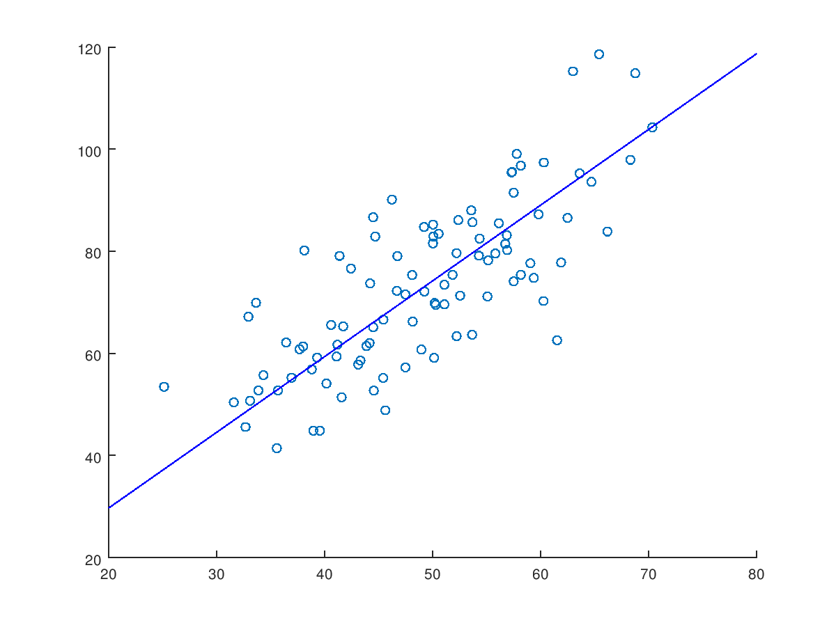Figure 2 – Linear regression result

A good way to debug the code is checking the error in every iteration. Here is the plot error vs iteration showing the error decreasing which is a good sign. After about 100 iterations the errors almost didn’t decrease.

Figure 3 – Error vs Iteration

We can see as well in every step how we improve our final curve. We started with a = b = 0 which is the x – axis. With the update of a and b, we notice the line goes up towards the cloud of points.

Figure 4 – Linear regression steps

What happens if we set a and b with different values at start? For example, starting  a = 100 \text{ and } b = -100 after 1000 iterations we would have:

Figure 5 – Not so optimal result

Although the error decreases and the algorithm converges, we can see that we actually found a local minimum since this line seems to split in half the set of points, but not in a optimal manner. We can even try with 10000 iterations and we’ll got the same result. So, start values for a and b can change the final result.

Tips

Here some tips:

1. Try different learning rates – \alpha. It makes the algorithm converge faster. If you error increases after some steps, try decreasing \alpha.
2. Try different start values for a and b, since you can find local minimum.
3. Test this code with different error function, play with different data, start point for a and b, test different values of alpha, understand the code and overall, have fun!

Conclusion

As we can see, linear regression is quite simple but powerful enough to solve simple problems. The most important thing is the concept which will be used for others algorithms that we’ll discuss later on the blog.

You can download this algorithm done in Octave from my github repository at https://github.com/marcelojo/simple_linear_regression.git

Marcelo Jo

Marcelo Jo is an electronics engineer with 10+ years of experience in embedded system, postgraduate in computer networks and masters student in computer vision at Université Laval in Canada. He shares his knowledge in this blog when he is not enjoying his wonderful family – wife and 3 kids. Live couldn’t be better.