Hi folks,
Yeah, things are getting more interesting, huh? In the last posts we covered linear regression where we fit a straight line to represent the best way possible a set of points. This is a simple and powerful way to predict values. But sometimes instead of predicting a value, we want to classify them.
Why we would do that? I know that is easy to understand but for those who didn’t catch it, why this is interesting?
We humans classify almost everything in our life without noticing it. We are able to recognize, differentiate and categorize stuffs. We know that a dog is a dog and not a wolf. We can recognize people, cars, buildings, etc. Now, imagine if we could make a program which is able to do the same, it wouldn’t be nice?
Classification
The classification problem is just like the regression problem, except that the values we now want to predict take on only a small number of discrete values. We’ll cover first binary classification problem which means that we have only two classes.
For example we could classify a house being expensive or not expensive depending on the number of rooms, area, price, city, etc.
Sigmoid function
In linear regression we were using h(x) = a_0x_0 + a_1x_1 + ... equation to fit the best curve given a set of points.
In logistic regression we don’t want to fit a curve in a set of points as in linear regression but instead classify data in categories. For that we’ll use the sigmoid function that is expressed as:
z = a_0x_0 + a_1x_1...
h(x) = g(z) = \dfrac{1}{1 + e^{-z}}
Having the following shape
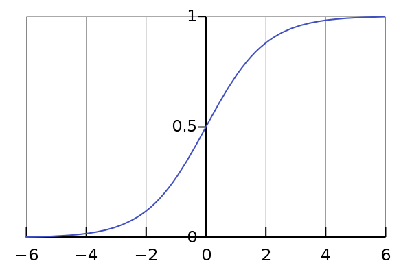
Figure 1 – Sigmoid function
This function is interesting since it maps any value of z into a number between 0 and 1. So h(x) will actually represents the probability that our output is 0 or 1, where 0 or 1 will be our two classes.
As our solution is discrete, we may “round” the result as follow:
h(x) \ge 0.5 \to y = 1
h(x) < 0.5 \to y = 0
Looking at Figure 1 we can see that at z = 0 we have y = 0.5 so:
z \ge 0 \to y = 1
z < 0 \to y = 0
where (again) z = a_0x_0 + a_1x_1... = a^Tx .
Now, if we pay attention, we have two inequalities. This means that now we have a curve and two regions. One when y = 0 and another when y = 1 which are our two possible classes.
It worth notice that z don’t need to be linear, it can be any polynomial function like z = a_0x_0 + a_1x_1^{2} + a_2x_0x_1.
Error minimization
As in linear regression, we must minimize the error. In logistic regression the error function is defined as
\displaystyle error = \frac{1}{m}\sum_{i=1}^{m} Cost(h(x), y) \text {\hspace{10 mm} \small eq. 1}
Where the cost function is
Cost(h(x) , y) = -log(h(x)) if y = 1
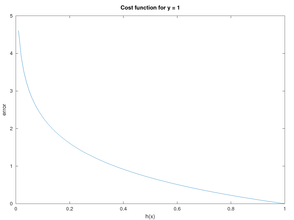 Figure 2 – Cost error for y = 1
Cost(h(x) , y) = -log(1 - h(x)) if y = 0
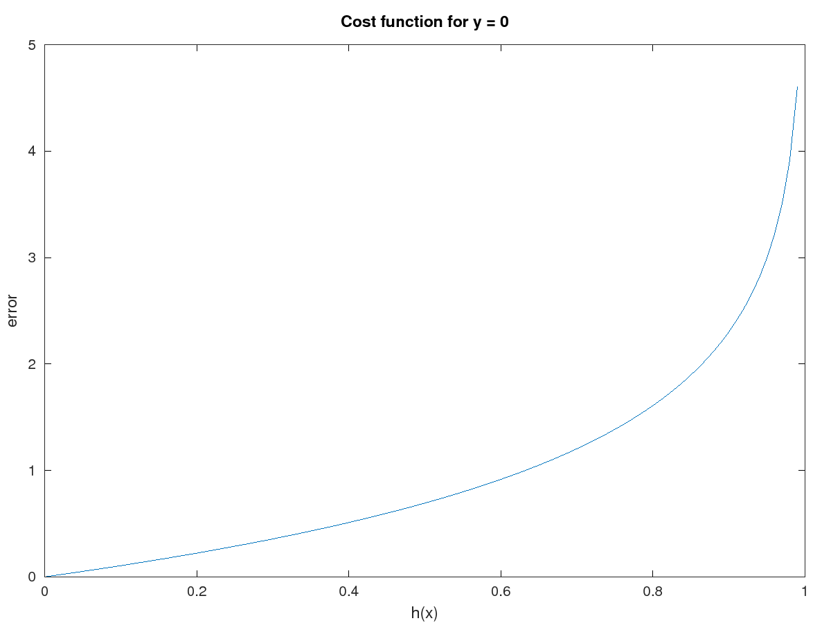 Figure 3 – Cost error for y = 0
This two cost functions above indicates that h(x) must be equal to y to have zero error. If not, the error will grow exponentially.
We can simplify and merge both equations into one like this
Cost(h(x),y) = -ylog(h(x)) - (1 - y)log(1 - h(x)) \text {\hspace{13 mm} \small eq. 2}
Note that using this equation guarantees that the error will be convex for logistic regression, which means we’ll converge to a global minimum when using gradient descent.
Finally our error function will be:
\displaystyle error = -\frac{1}{m}\sum_{i=1}^{m}[ylog(h(x)) + (1 - y)log(1 - h(x))] \text {\hspace{10 mm} \small eq. 3}
Gradient descent
As in linear regression, we can use gradient descent to minimize the error function (eq 3) and find the constants a_n .
We still need to calculate the derivatives and follow the same algorithm.
\displaystyle \frac{\partial error}{\partial a_n} = -\frac{1}{m}\sum_{i=1}^{m} x_n \left ( h(x) - y) \right ) \text {\hspace{10 mm} \small eq. 4}
In each iteration we must update parameters as we did in linear regression
\displaystyle new \textunderscore a_n = a_n - \alpha\frac{\partial}{\partial a_n} \text {\hspace{25 mm} \small eq. 5}
Conclusion
In this post we covered the theory of logistic regression which is very close to linear regression. Besides the name, it’s a classification algorithm which allow us to classify data in two different classes.
In the next post we’ll get our hands dirty and testing this algorithm to classify some data and check how it will perform.
Seeya!!!
Marcelo Jo is an electronics engineer with 10+ years of experience in embedded system, postgraduate in computer networks and masters student in computer vision at Université Laval in Canada. He shares his knowledge in this blog when he is not enjoying his wonderful family – wife and 3 kids. Live couldn’t be better.

 I'm an electronics engineer with 10+ years of experience in embedded system, hardware and firmware development for several 8/16/32 bits microcontrollers like 8051, Microchip, MSP430, Freescale, ARM, etc. I'm a passionate in electronics and embedded systems, but not a nerds! =P


Leave a Reply